
opencvのlaplacian、numpy、skimage laplacianを使った画像処理をテストしてみた。
スポンサーリンク
ラプラシアンフィルタ(opencv編)
先ずはテスト用の画像イメージを下記サイトからダウンロードする。
%download http://aishack.in/static/img/tut/sudoku-original.jpg
import cv2
import numpy as np
from matplotlib import pyplot as plt
import matplotlib.pylab as pylab
pylab.rcParams['figure.figsize'] = 30, 20
pylab.rcParams["font.size"] = "30"

img = cv2.imread('sudoku-original.jpg',0)

laplacian = cv2.Laplacian(img,cv2.CV_64F)
sobelx = cv2.Sobel(img,cv2.CV_64F,1,0,ksize=5)
sobely = cv2.Sobel(img,cv2.CV_64F,0,1,ksize=5)

plt.subplot(1,4,1),plt.imshow(img,cmap = 'gray')
plt.title('Original'), plt.xticks([]), plt.yticks([])
plt.subplot(1,4,2),plt.imshow(laplacian,cmap = 'gray')
plt.title('Laplacian'), plt.xticks([]), plt.yticks([])
plt.subplot(1,4,3),plt.imshow(sobelx,cmap = 'gray')
plt.title('Sobel X'), plt.xticks([]), plt.yticks([])
plt.subplot(1,4,4),plt.imshow(sobely,cmap = 'gray')
plt.title('Sobel Y'), plt.xticks([]), plt.yticks([])
plt.show()
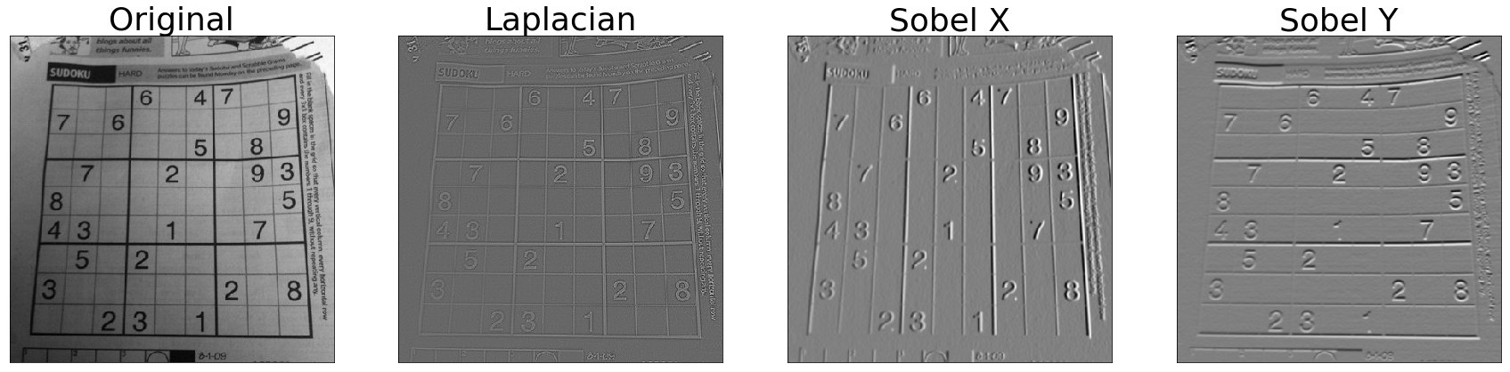
画像が以下のチュートリアルの画像とは違うので修正を試みた。
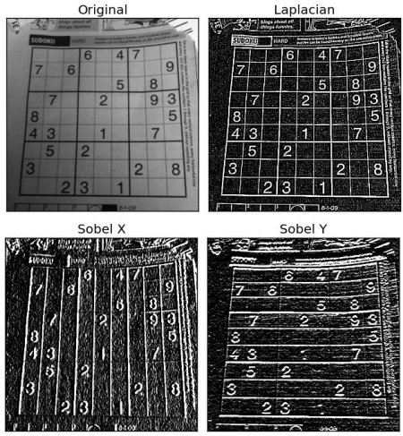
%download https://docs.opencv.org/3.0-beta/_images/gradients.jpg
from IPython.display import Image, display
display(Image("gradients.jpg"))
import cv2
import numpy as np
from matplotlib import pyplot as plt
import matplotlib.pylab as pylab
pylab.rcParams['figure.figsize'] = 30, 20
pylab.rcParams["font.size"] = "30"

img = cv2.imread('sudoku-original.jpg',0)

laplacian = cv2.Laplacian(img,cv2.CV_64F)
sobelx = cv2.Sobel(img,cv2.CV_64F,1,0,ksize=5)
sobely = cv2.Sobel(img,cv2.CV_64F,0,1,ksize=5)

plt.subplot(1,4,1),plt.imshow(img,cmap = 'gray')
plt.title('Original'), plt.xticks([]), plt.yticks([])
plt.subplot(1,4,2),plt.imshow(laplacian,cmap = 'gray', vmin=0, vmax=20)
plt.title('Laplacian'), plt.xticks([]), plt.yticks([])
plt.subplot(1,4,3),plt.imshow(sobelx,cmap = 'gray', vmin=0, vmax=512)
plt.title('Sobel X'), plt.xticks([]), plt.yticks([])
plt.subplot(1,4,4),plt.imshow(sobely,cmap = 'gray', vmin=0, vmax=512)
plt.title('Sobel Y'), plt.xticks([]), plt.yticks([])
plt.show()
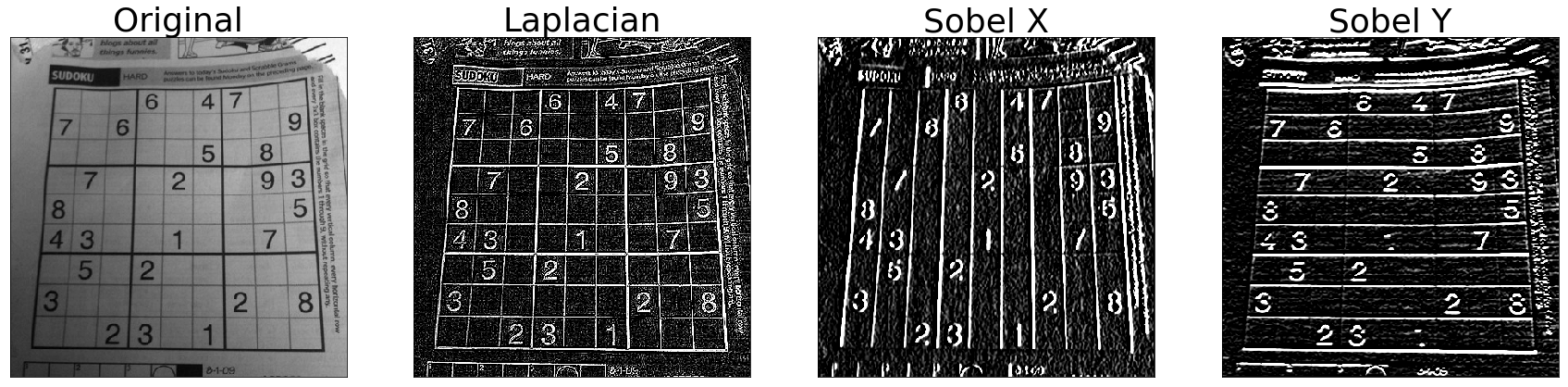
vmin/vmaxオプションを調整することで画像をチュートリアルのようにできた。
スポンサーリンク
ラプラシアンフィルタ(skimage編)
テストに必要なモジュールをインポートする。
import skimage.color
from skimage.filters import laplace
import numpy as np
image = img
image = skimage.color.rgb2gray(image)
image.shape
def laplace_skimage(image):
    """Applies Laplace operator to 2D image using skimage implementation.
    Then tresholds the result and returns boolean image."""
    laplacian = laplace(image)
    thresh = np.abs(laplacian) > 0.05
    return thresh
edges = laplace_skimage(image)
edges.shape
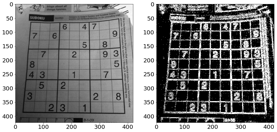
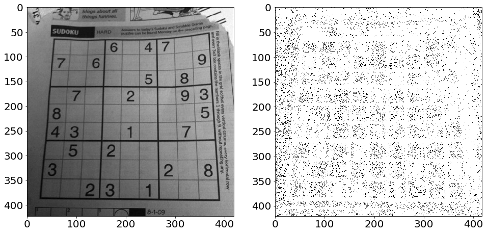
def compare(left, right):
    """Compares two images, left and right."""
    pylab.rcParams["font.size"] = "20"
    fig, ax = plt.subplots(1, 2, figsize=(16, 8))
    ax[0].imshow(left, cmap='gray')
    ax[1].imshow(right, cmap='gray')
compare(left=image, right=edges)
スポンサーリンク
ラプラシアンフィルタ(numpy編)
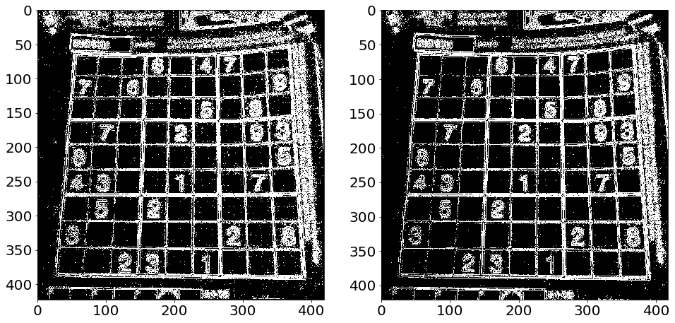
def laplace_numpy(image):
    """Applies Laplace operator to 2D image using our own NumPy implementation.
    Then tresholds the result and returns boolean image."""
    laplacian = image[:-2, 1:-1] + image[2:, 1:-1] + image[1:-1, :-2] + image[1:-1, 2:] - 4*image[1:-1, 1:-1]
    thresh = np.abs(laplacian) > 0.05
    return thresh
laplace_numpy(image).shape
compare(image, laplace_numpy(image))
np.allclose(laplace_skimage(image)[1:-1, 1:-1], laplace_numpy(image))
画像はどう見ても違うが、np.allcloseはtrueなので間違いではなさそうだ。因みに、画像は以下のようにすると同じようなものに仕上がる。
def laplace_numpy(image):
    """Applies Laplace operator to 2D image using our own NumPy implementation.
    Then tresholds the result and returns boolean image."""
    laplacian = image[:-2, 1:-1] + image[2:, 1:-1] + image[1:-1, :-2] + image[1:-1, 2:] - 4*image[1:-1, 1:-1]
    thresh = np.abs(laplacian) > 15
    return thresh

compare(edges, laplace_numpy(image))
次回は、skimage, numpy, cv2の処理速度比較をやってみたい。
スポンサーリンク