
庶民に優しい民主党政権の円高時、1kg1000円程度で買えていたネットで高評価の無塩ローストアーモンドが、安倍政権下で断行された増税・円安政策(いわゆる世に言うアベノミクス)のせいで、1kg2000円以上に跳ね上がった。庶民いじめ以外の何物でもないアホノミクスの愚策により食品価格は、民主党政権時に比べ、軒並み1.5倍〜3倍に暴騰している。10月にさらに消費税が上がれば、軽減税率などどこ吹く風で食品価格は上昇を続け、日本人の8割を占める庶民の生活は完全に破壊されるだろう。閑話休題、日本がどのくらいアメリカからアーモンドを輸入しているのかをグラフ化する。
from pandas import *
import warnings
warnings.simplefilter('ignore', FutureWarning)
from pandas import *
import matplotlib
matplotlib.rcParams['axes.grid'] = True # show gridlines by default
%matplotlib inline

df = read_csv('usa_almond.csv',encoding='utf-8')
df.head(2)
df=df[['Year', 'Period','Trade Flow','Reporter', 'Partner', 'Commodity','Commodity Code','Netweight (kg)','Trade Value (US$)']]
df2=df.groupby(['Commodity','Commodity Code'])
df2['Netweight (kg)'].aggregate(sum)
in shellは殻付き、shelledは殻なしの意味。
スポンサーリンク
米国の日本へのアーモンド輸出額推移
df1 = df[['Period','Trade Value (US$)']].sort_values(by='Period',ascending=True)
group = df1.groupby('Period')
g1 = group['Trade Value (US$)'].aggregate(sum)
g2 = DataFrame(g1).sort_values(by='Period',ascending=False)
from matplotlib.pyplot import *
from matplotlib.font_manager import FontProperties
from matplotlib import rcParams
import matplotlib.patches as mpatches
style.use('ggplot')

rcParams["font.size"] = "18"
fp = FontProperties(fname='/usr/share/fonts/opentype/ipaexfont-gothic/ipaexg.ttf', size=54)
rcParams['font.family'] = fp.get_name()

rcParams["font.size"] = "25"
fig, ax = subplots(figsize=(22,15))
g2.plot(ax=ax, kind='barh',width=.8,color='pink',legend=False)
rc('xtick', labelsize=25)
rc('ytick', labelsize=25)
xticks(np.arange(0,3.3e8,1e8/5),
 ['{}千万'.format(int(x/1e7)) if 1e8> x > 0 else '{}億'.format(float(x/1e8)) if \
  x >= 1e8 else 0 for x in np.arange(0,3.3e8,1e8/5)])
ax.legend(["輸出額"],loc='best', prop={'size': 26})
for j,i in enumerate(ax.patches):
    ax.text((i.get_width()+9e5 if int(i.get_width()) < 2.9e8 else i.get_width()-6.5e7),\
     i.get_y()+.1,'{:,}億{:,}万{:,}ドル'.format(int(str(i.get_width())[:-8]),\
       int(str(i.get_width())[-8:-4]),int(str(i.get_width())[-4:])) \
 if int(i.get_width()) > 1e8 else '{:,}万{}ドル'.format(int(str(i.get_width())[-8:-4]),int(str(i.get_width())[:-4])),\
            fontsize=20, color='k');
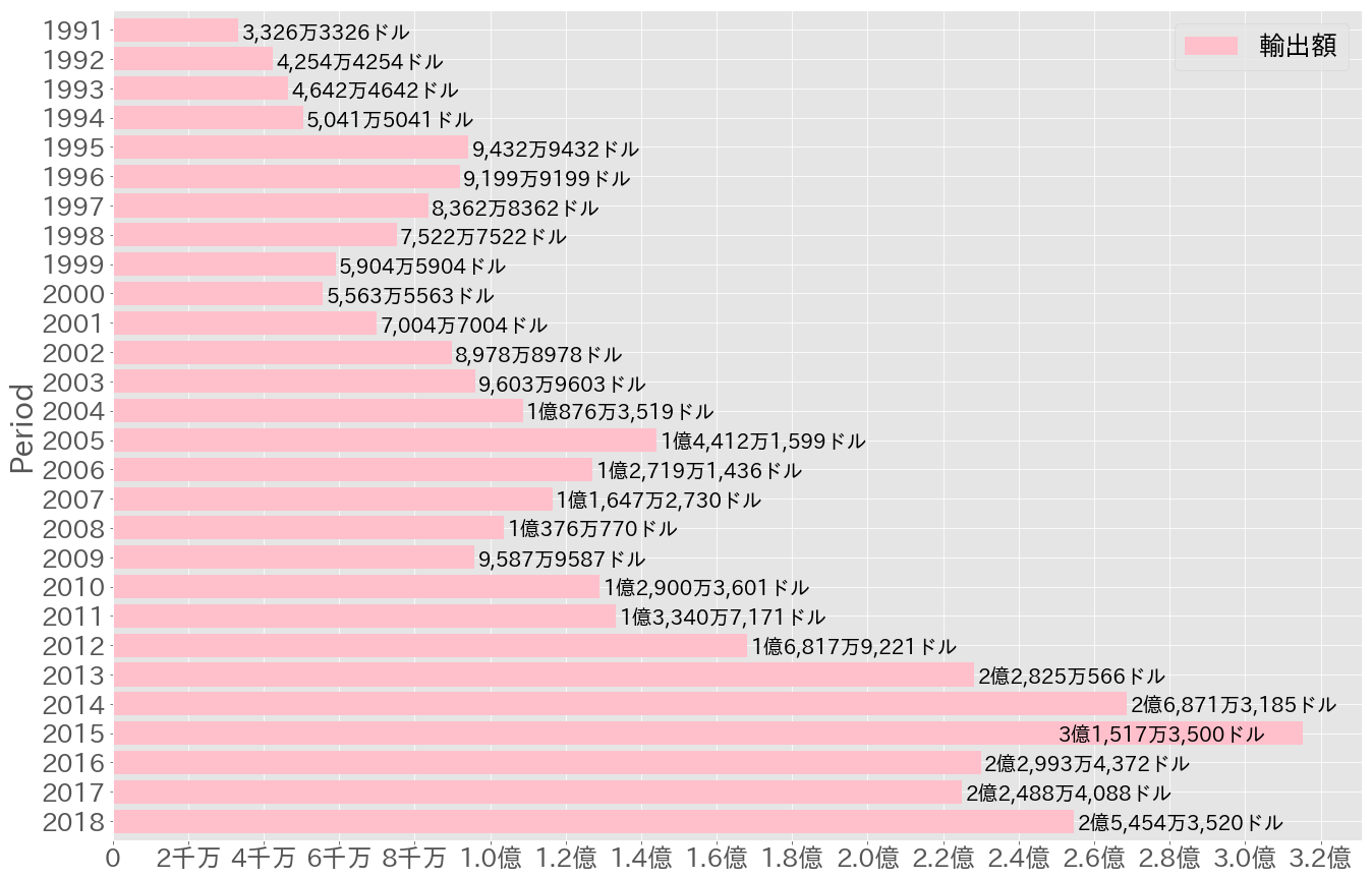
2004年に初めて1億ドルの大台を超えて以来、2009年の世界大不況を別にすれば、コンスタントに1億ドル台を維持し続けている。今度は輸出量で見てみる。
スポンサーリンク
米国の日本へのアーモンド輸出量推移
df2 = df[['Period','Netweight (kg)']].sort_values(by='Period',ascending=True)
group = df2.groupby('Period')
g3 = group['Netweight (kg)'].aggregate(sum)
g4 = DataFrame(g3).sort_values(by='Period',ascending=False)
from matplotlib.pyplot import *
from matplotlib.font_manager import FontProperties
from matplotlib import rcParams
import matplotlib.patches as mpatches
style.use('ggplot')

rcParams["font.size"] = "18"
fp = FontProperties(fname='/usr/share/fonts/opentype/ipaexfont-gothic/ipaexg.ttf', size=54)
rcParams['font.family'] = fp.get_name()

rcParams["font.size"] = "25"
fig, ax = subplots(figsize=(22,15))
g4.plot(ax=ax, kind='barh',width=.8,color='pink',legend=False)
rc('xtick', labelsize=25)
rc('ytick', labelsize=25)
xticks(np.arange(0,4.6e7,1e7/2),
 ['{}万'.format(int(x/1e4)) if 1e8> x > 0 else '{}億'.format(float(x/1e8)) if \
  x >= 1e8 else 0 for x in np.arange(0,4.6e7,1e7/2)])
ax.legend(["輸出量"],loc='best', prop={'size': 26})
for j,i in enumerate(ax.patches):
    ax.text((i.get_width()+1e5 if int(i.get_width()) < 4e7 else i.get_width()-0.8e7),\
     i.get_y()+.1,'{:,}億{:,}万{:,}kg'.format(int(str(i.get_width())[:-8]),\
       int(str(i.get_width())[-8:-4]),int(str(i.get_width())[-4:])) \
 if int(i.get_width()) > 1e8 else '{:,}万{}kg'.format(int(str(i.get_width())[-8:-4]),int(str(i.get_width())[:-4])),\
            fontsize=20, color='k');
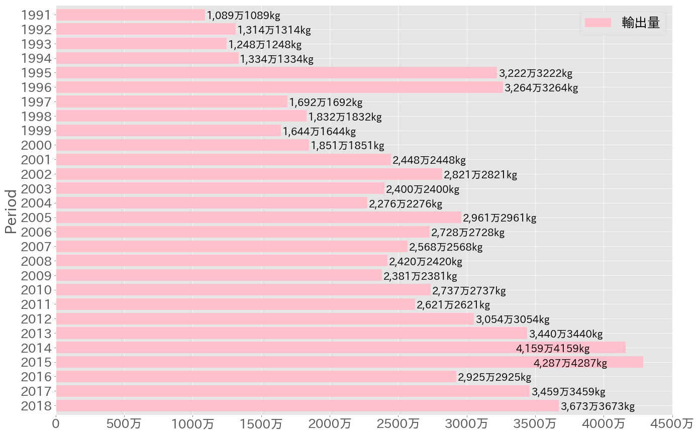
1991年と2015年を比べると、金額ベースだと10倍近いのに、重量ベースだと4倍なのは、それだけアーモンド価格が値上がっているということである。1996年と2015年は重量ベースだと1000万kg(1万トン)しか違わないのに、金額ベースだと2億ドル以上違う。何でこの2年間だけこんなに日本のアーモンドの輸入量が多いのかは知らんが、1997年の消費税増税や1995年に1ドル80円になったことと関係があるかもしれん。
print(91998909/32642035)
print(315173500/42873712)
1996年は2.81842ドル/kgだったアーモンドが、2015年には7.35121ドルに値上がっている。値上がり率は、この間のアメリカのGDP成長率にほぼ等しいと思われる。
スポンサーリンク